EPViz (EEG Prediction Visualizer)

EPViz is a tool to aid researchers in developing, validating, and reporting their predictive modeling outputs. A lightweight and standalone software package developed in Python, EPViz allows researchers to load a PyTorch deep learning model, apply it to the EEG, and overlay the output channel-wise or subject-level temporal predictions on top of the original time series.

For installation, please visit our Github or PyPI pages. Alternatively, you can download our standalone app for MacOS and Windows here.

Features

Loading signals in average reference and longitudinal bipolar montages
Loading files with a custom montage
High pass and low pass filtering of the EEG signals
Applying PyTorch models to data to produce predictions
Loading PyTorch predictions produced by an auxiliary model
Saving the EEG signals to an EDF file with an option to anonymize the data
Saving high quality images of the EEG signals and predictions
A Topoplot viewer for channel-wise predictions
Computing basic signal statistics
Spectrogram computation and analysis
Annotation editor

Demo Video

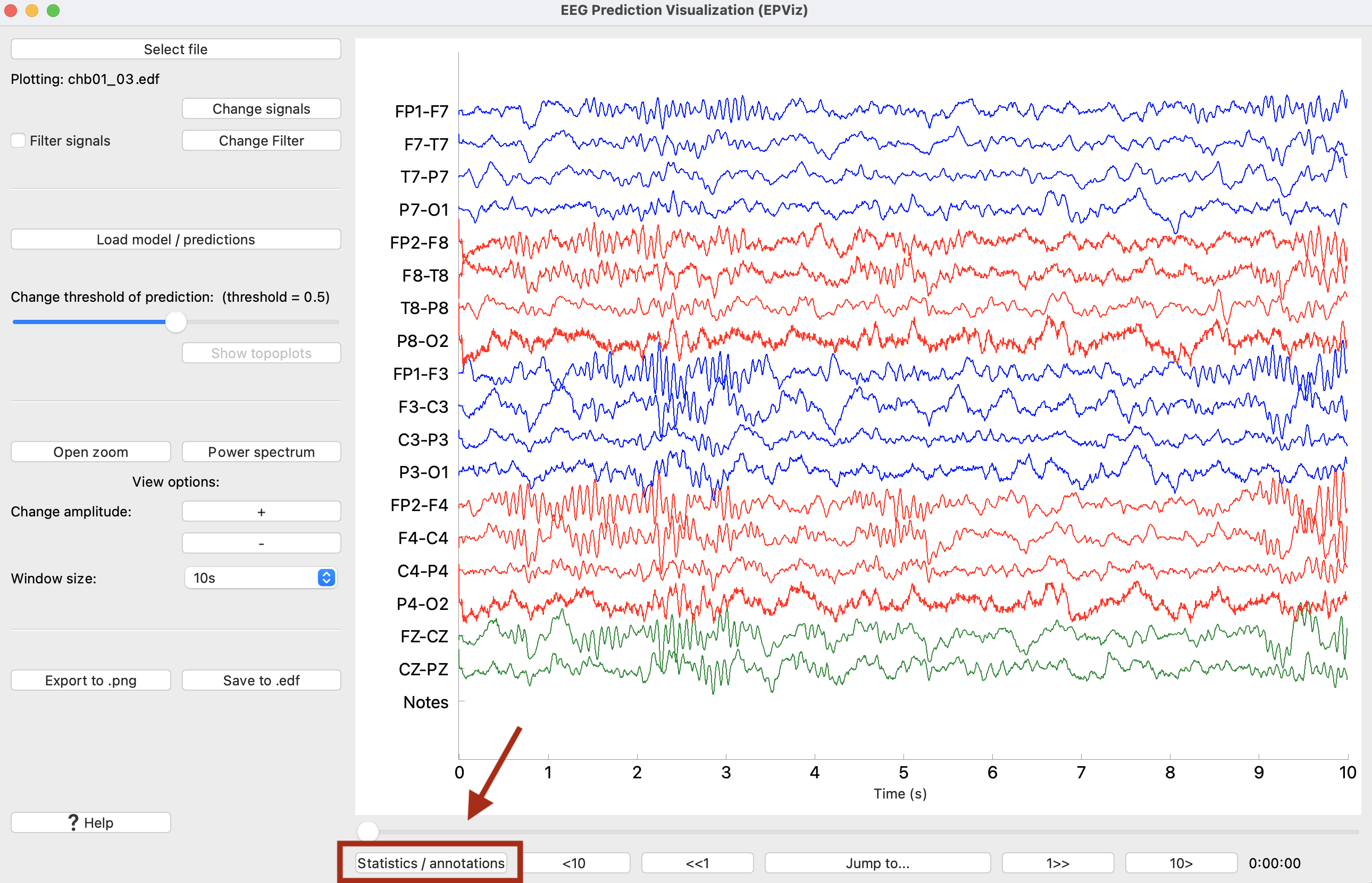
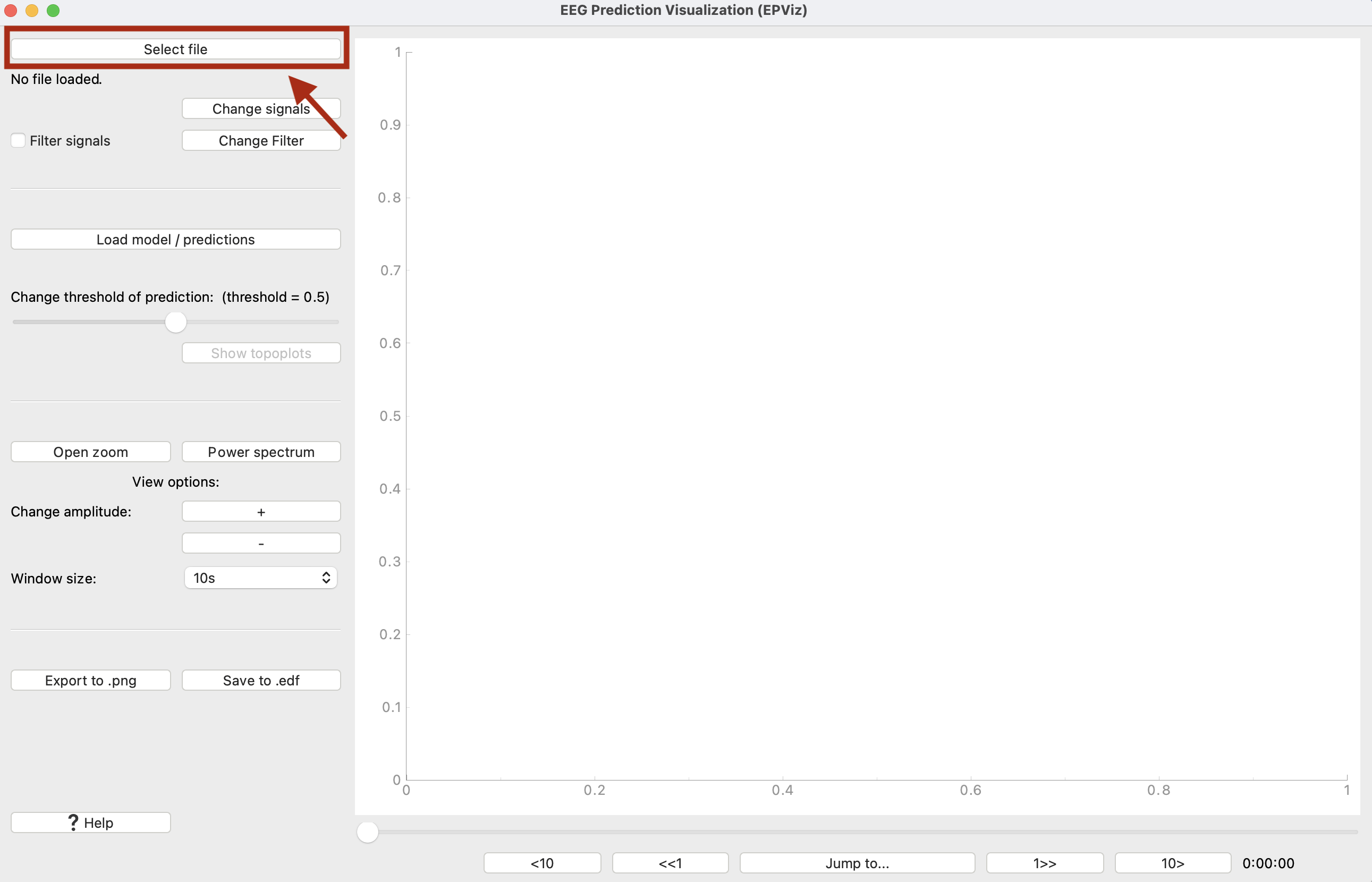
0) Main window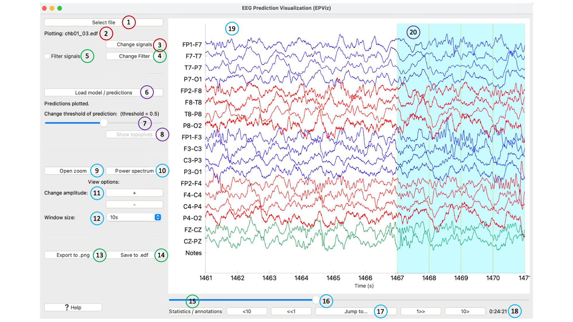 ① Select an EDF file to load
② Shows the name of the loaded EDF file
③ Click to change which signals are plotted, add a custom montage, change the signal colors or ordering
④ Edit the filter parameters
⑤ Toggle to turn the filter on or off
⑥ Opens a window to load model predictions
⑦ Slider changes the threshold above which predictions will be shown in light blue
⑧ If channel-wise predictions are plotted, this button will be enabled and will open the topoplot sidebar for alternate visualization
⑨ Opens a zoomed in window of the signals
⑩ Opens the editor to show spectrograms
⑪ Scales signals making amplitudes larger or smaller for viewing
⑫ Change the number of seconds displayed at one time
⑬ Save the main window as a high quality *.png file
⑭ Save the signals to an EDF file, with the option to anonymize the file
⑮ Open the right sidebar to show the annotation editor and signal statistics
⑯ Slider to change what part of the signals are shown
⑰ Jump to a certain time in the recording
⑱ The time shown in the plot window in hours:minutes:seconds
⑲ The main plot window where signals are shown
⑳ Model predictions are displayed in blue

To load signals, click the “Select file” (①) button at the top of the left sidebar. Choose the EDF file you would like to view. Next, the “Select signals” window will appear, as shown below. The 10-20 average reference and bipolar montages have been preconfigured and will appear as checkboxes when available. You may also load a custom list of signals. A test file called “test_chns.txt” is loaded in the image below.

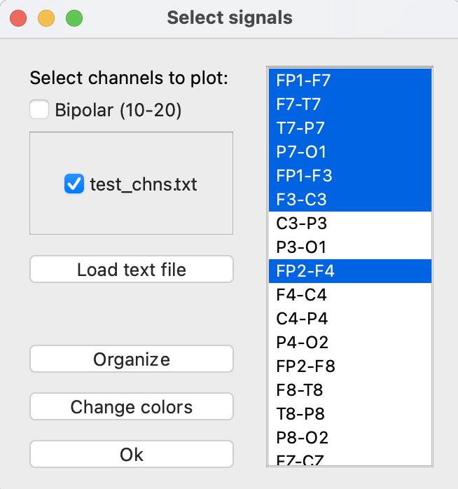
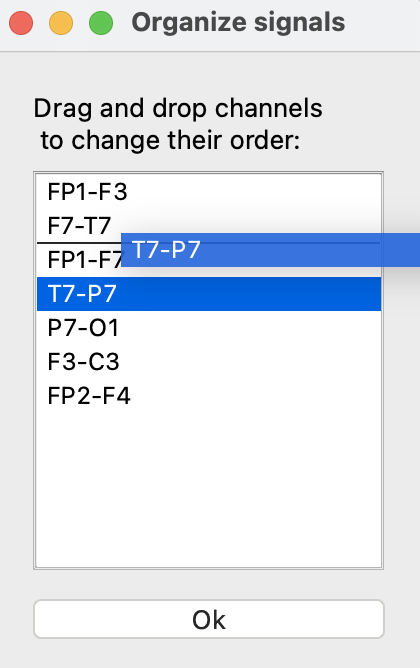
The signals are loaded in the order specified by the EDF header. The “Organize” button can be used to change the ordering. In this window, signals can be dragged and dropped into a different order. Note that if a custom file is loaded, signals will be ordered by default according to the text file but can be reordered using this window.

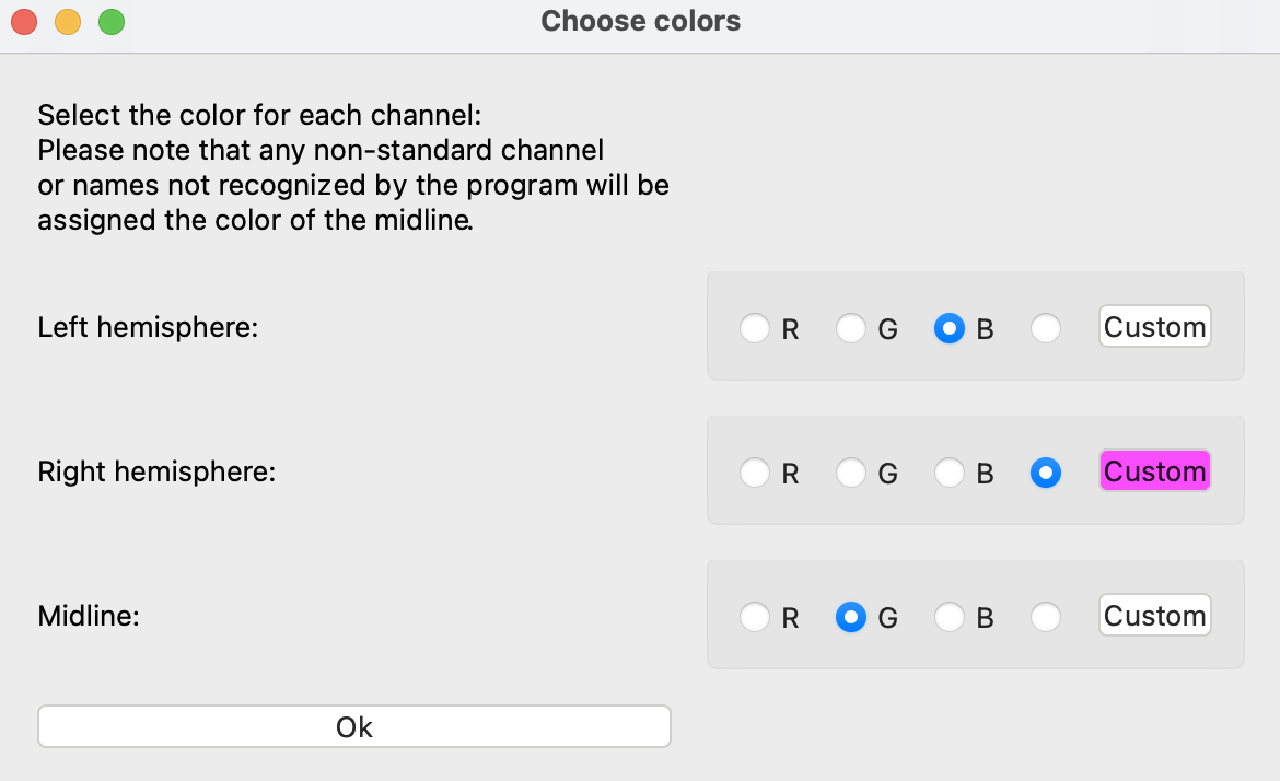
Finally, the “Change colors” button allows you to select the EEG signal colors used for plotting. The signals have been grouped into left hemisphere, right hemisphere, and midline. The default is left will be blue, right will be red, and midline will be green. Any channels that are not recognized as falling into these groups will be plotted in green. To pick a custom color, click the “Custom” button and select a color from the color picker. To apply it to the data, select the radio button next to “Custom”.

In the example shown below, right channels will be shown in a custom pink color.

Tips for using the signal selection:

If the bipolar and average reference options are not showing for your file, it is likely because your channels are not named according to the standard convention. Please rename the channels in your EDF file and try again.
Custom montage files must have channel names that either match the EDF header or follow the standard 10-20 naming convention.
Custom montage files must have a single channel per line. To see an example of how to format your text file, please check out our Github repo.
The maximum channels that can be plotted at once is 70.

2) Loading models and predictions

To load a model and predictions, select the “Load model / predictions” button (⑥). There are two ways to load predictions in EPViz:

1) Load predictions as a single Pytorch (.pt) file. Predictions must be of shape (number of samples, number of channels (optional), predictions for each class).

2) Load a pretrained model (as a PyTorch (.pt) file) and a separate file that contains the preprocessed data features. The features will be passed through the model and the resulting predictions will be plotted. This setup allows the user to separately compute features from the EEG data prior to evaluation and plotting.

Binary predictions should be in the range [0,1]. The user can sweep the threshold slider to customize the range of predictions that will be overlaid in blue on the plot. Multi-class predictions should be output as a softmax vector matching the number of classes. By default the maximum value will be used as the class label and overlaid on the EEG. Each class will be plotted in a different color.

Both options (1) and (2) can be loaded at once. By toggling the checkbox to the left of each option, the user can toggle whether or not predictions are plotted. Predictions will be maintained until they are overwritten or the session ends.

Tips for loading predictions:

Must be PyTorch (.pt) files, other file types are not supported at this time.
You can load either predictions OR preprocessed data and a model
The prediction output is assumed to be for non-overlapping intervals of constant width. Formally, the length of the prediction output should be an integer factor of the number of time samples in the EDF file.
Channel-wise predictions will be plotted starting from the top of the screen
Predictions are assumed to be binary with classes 0 and 1. If you would like to plot more than two classes, select the “multi-class” option.
For multi-class predictions, the output must be of size (integer factor of EDF samples, num chns (optional), num classes)

3) Saving figures

To save the plot window, select the “Export to png” (⑬) button. This will open an editor where the annotations can be toggled on or off, the font size can be edited, the signal thickness can be changed, and a title can be added.

If multi-channel predictions are plotted, then the topoplots pane will be enabled. The topoplot figures can be saved by clicking the “Save topoplot images” button located at the bottom of the topoplot dock. This will load images for each topoplot frame shown in the main plotting window. In the editor, timestamp titles can be added and either all images or a single frame can be plotted.

Topoplots are generated using the MNE package. For more information, please visit their website: https://mne.tools/dev/generated/mne.viz.plot_topomap.html.

4) Saving to EDF

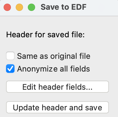
To save to an EDF file, click the “Save to edf” (⑭) button. This will open a selection window shown below. This window allows the user to either keep the EDF header information from the original file, or to anonymize all fields. Select one of these options, and click the “Update header and save”. This will prompt the user to select a location for the file to be saved and produce the output EDF file. The user can also edit individual header fields prior to saving by clicking the “Edit header fields…” button.

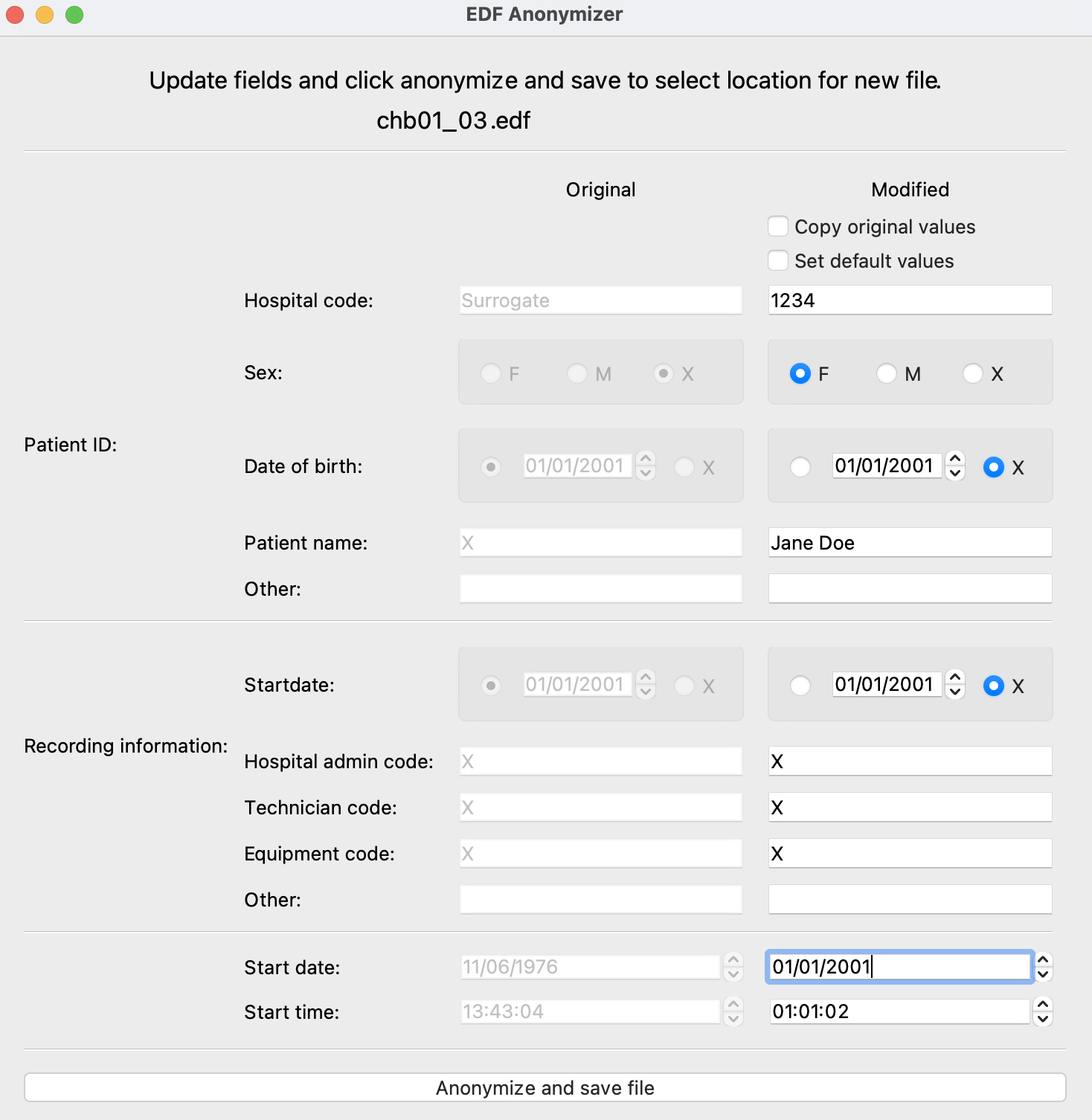
After selecting “Edit header fields” the full Anonymizer module will open as illustrated below. The original header values are shown in the left column and the modified versions are shown in the right column. The user can copy the original values by selecting the appropriate checkbox at the top. The user may also use our default anonymization protocol or edit the individual fields. The content of the right column will be saved to the new EDF file when the “Anonymize and save file” button is clicked.

Tips for saving EDF files:

If any of the required fields are left blank in the Anonymization pane, they will be filled with the default value of “X”
If filtering is turned on, filtered signals will be saved to the EDF file. An annotation will be added to EDF that the signals are filtered and the filter parameters.
If predictions are turned on, they will be saved to the EDF file as a separate channel called “PREDICTIONS” (patient-level) or “PREDICTIONS_i” (channel-wise) where i is an integer for each of the i channels.
Only channels that are currently plotted on the main viewer will be saved.

5) Annotation editor

The annotation editor allows the user to create, update, or delete annotations. If there are annotations in the loaded file (e.g., clinical notes), they will appear in the right sidebar. Otherwise, the annotation sidebar can be opened via the “Statistics / annotations” button found below the main plot as shown in the image below.

Once opened, the annotation editor allows the user to update (overwrite) existing annotations, delete an annotation, and create (add) a new annotation. Each annotation has 3 properties: text, time, and duration. In the annotation editor time is shown in two formats: hours, minutes, and seconds (hh:mm:ss) on the left and seconds on the right. When editing time in one format, the other will automatically update for consistency. Clicking on an annotation in the list will take you to that time point in the EEG.

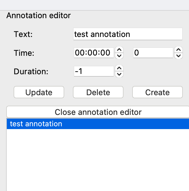
Tips for using the annotation editor:

Changes to annotations will not be preserved across sessions unless the result is saved to a new EDF file.
The annotation sidebar cannot be collapsed unless there are no annotations.

6) Filtering the EEG signals

Click the “Change filter” button near the top of the left side panel. Here, you can add low, high, or band pass filters. To apply the filter, toggle the “Filter signals” checkbox.

7) Signal statistics

Signal statistics can be found in the annotation sidebar. If the sidebar is closed because there are no annotations, it can be opened via the “Statistics / annotations” button. To view signal statistics, click the “Open signal stats” button. This will open a window with signal mean, variance, and line length, as well as energy in various frequency bands. Values are shown for the entire signal and a slideable region via to the red bar. 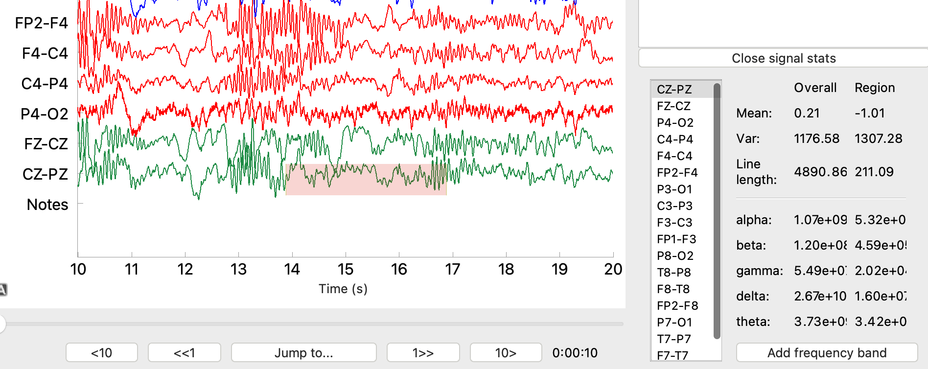Statistics can only be viewed for one EEG signal at a time. This is controlled by selecting the corresponding channel from the signal list in the signal stats pane. The region selector can be moved forwards and backwards in time. It can also be expanded and contracted by clicking and dragging on the edges of the highlighted region

The default frequency bands for the statistic computation are:

alpha (8 – 14 Hz)
beta (14 – 30 Hz)
gamma (30 – 45 Hz)
delta (1 – 4 Hz)
theta (4 – 8 Hz)

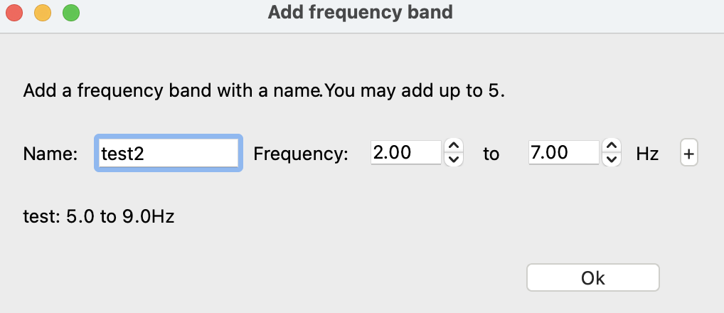
To add a custom frequency band, click “Add a frequency band.” This will open the window shown below. After typing in a name and two frequencies, click the “+” and then “Okay” to add this new band. You may add up to five custom bands.

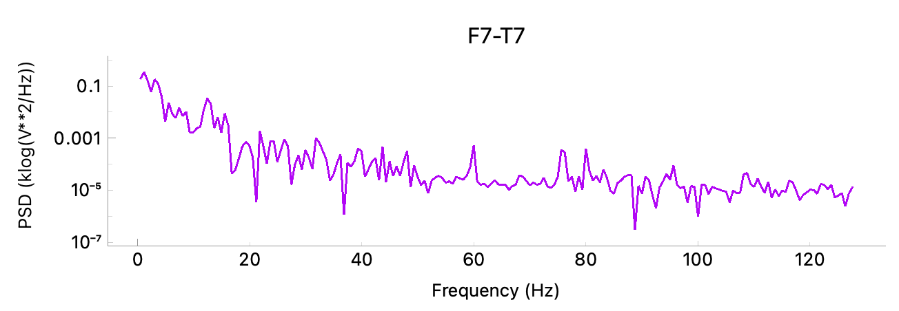
8) Power spectrum

To view the power spectrum for an EEG channel, click the “Power spectrum” button. Select a channel and the frequency range in Hertz to plot.

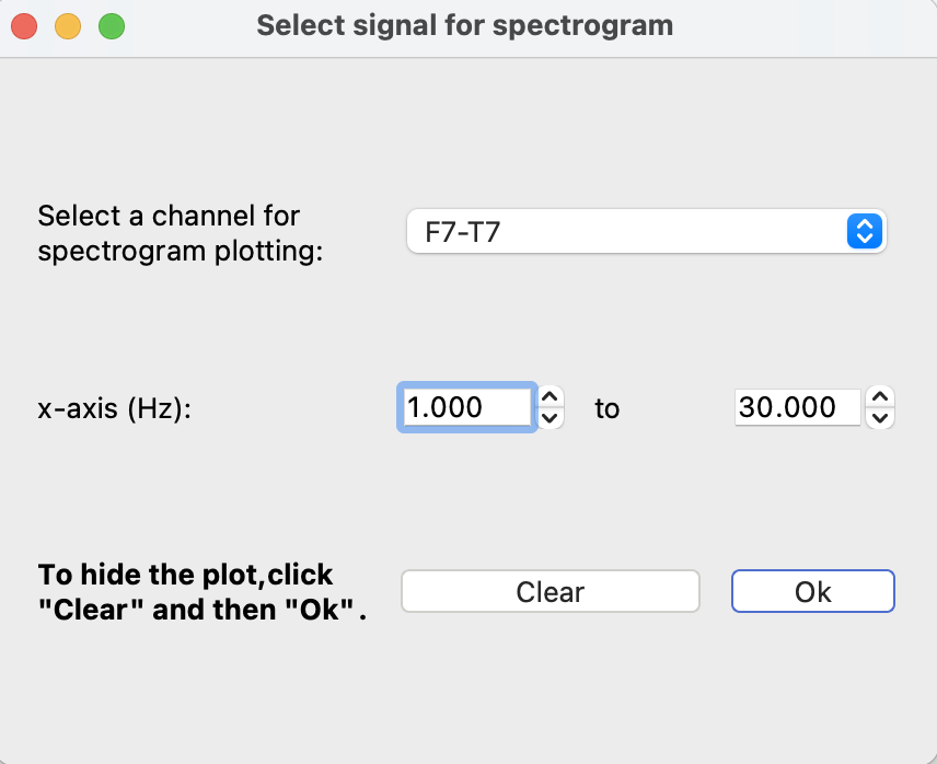
A red selection window will appear which can be used to choose the time interval. The graph will update as you move the selection window or the main plot. To close the graph, select “Power spectrum” and then “Clear” to clear the selected channel.

9) Plot settings

There are several buttons that can be used to customize the main viewing pane. On the left panel, the “Change amplitude” buttons will change the scale of the y-axis to make signals appear larger or smaller in amplitude. “Window size” refers to the number of seconds shown in the main plot which can be changed.

Finally, the “Open zoom” button will add an orange rectangular selection to the main viewing pane. The content inside this rectangle will be magnified. The rectangle can also be resized and dragged around to view different areas of the signal. To close this window, select the same button, which will now say “Close zoom.”

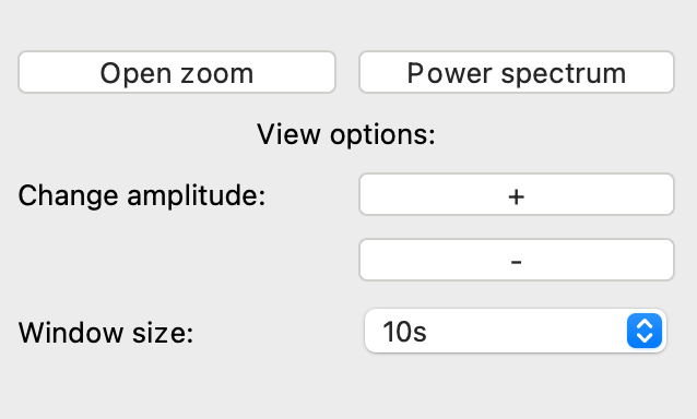
Below the main viewing pane are several buttons to move the plot in time. The slider will scroll the plot in real time. The “<10” and “<<1” buttons will jump backwards in time by 10 or 1 second increments, respectively. Likewise, the “10>” and “1>>” buttons will jump forwards in time. To go to a certain time point in the plot, click the “Jump to” button and enter the time in seconds where you would like to go. The time at the right converts seconds to hours, minutes and seconds specified by (hh:mm:ss).

10) Command line options

We have added command line options for batched processing and streamlined use:

$ python visualization/plot.py --show {0 | 1} --fn [EDF_FILE] --montage-file [TXT_FILE] --predictions-file [PT_FILE] --prediction-thresh [THRESH] --filter {0 | 1} [LOW_PASS_FS] [HIGH_PASS_FS] [NOTCH_FS] [BAND_PASS_FS_1] [BAND_PASS_FS_2] --location [INT] --window-width {5 | 10 | 15 | 20 | 25 | 30} --export-png-file [PNG_FILE] --plot-title [TITLE] --print-annotations {0 | 1} --line-thickness [THICKNESS] --font-size [FONT_SIZE] --save-edf-fn [EDF_FILE] --anonymize-edf {0 | 1}

For these options, 0 means off / False and 1 means on / True. These options include:

--show Whether or not to open the visualizer
--fn The .edf file to load
--montage-file What montage text file to use
--predictions-file Predictions to load
--prediction-thresh Threshold to use for the predictions (Default: 0.5)
--filter Filter specifications (on or off, and the frequencies in Hz for each filter) (Default: [0, 30, 2, 0, 0, 0])
--location Where in time to load the graph (Default: 0)
--window-width How many seconds to show in the window (Default: 10)
--export-png-file Name of .png file to save the graph
- --plot-title The title of the saved graph (Default: “”)
- --print-annotations Whether to show annotations on the saved graph (Default: 1)
- --line-thickness Line thickness of the saved graph (Default: 0.5)
- --font-size Font size for the saved graph (Default: 12)
--save-edf-fn Name of the .edf file to save
- --anonymize-edf Whether or not to anonymize the file (Default: 1)

If --fn is provided then --montage-file must be provided as well.

11) Demo

This demo will use the tuh_with_annotations.edf and the tuh_predictions.pt files found in the /test_files folder of our Github repository. Please note that these are “fake” predictions used for demo purposes only. Open the visualizer (if you have installed via pip, type “epviz” on the command line). First, let’s load the file. Click “Select File.”

Next, select “Average reference (10-20)” as our montage and click “Ok” to plot the EEG.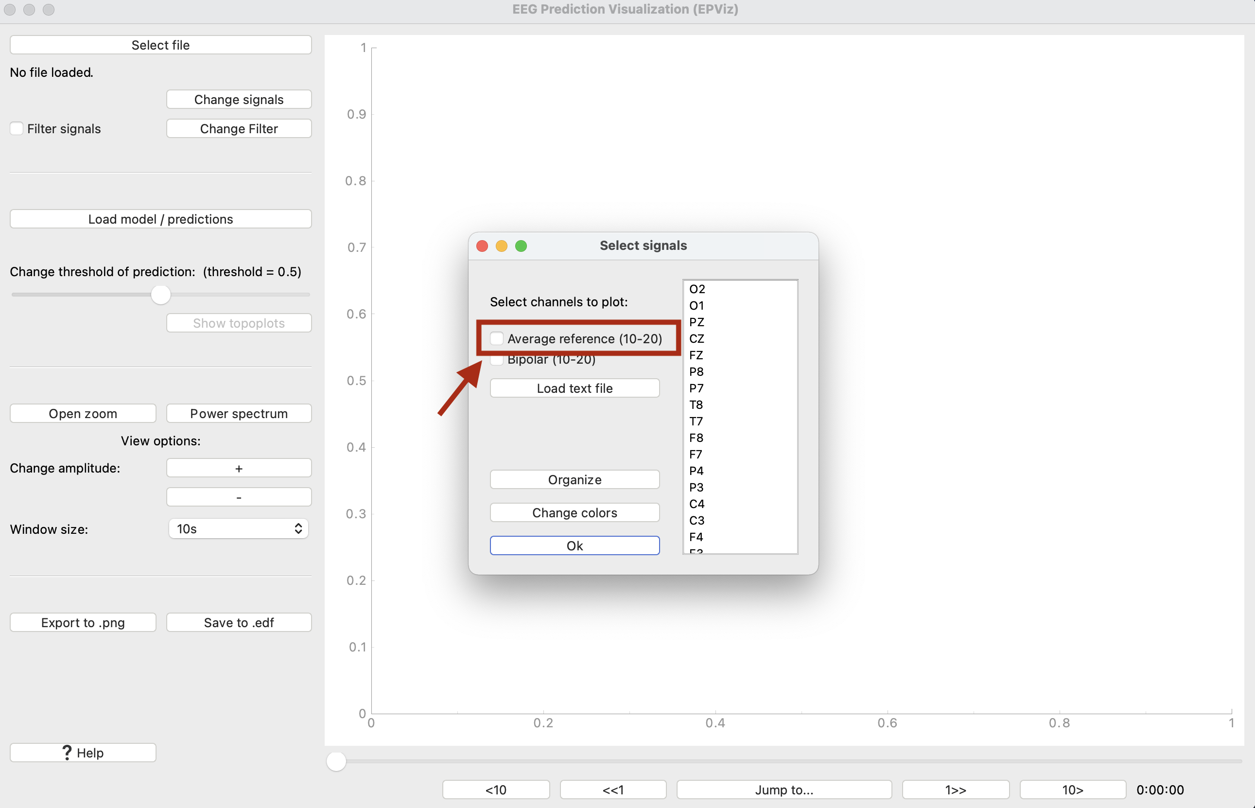

We can see that the signals have been loaded, and the annotations have been populated in the right sidebar. From here, we want to load predictions. Select “Load model / predictions” to load in the PyTorch file.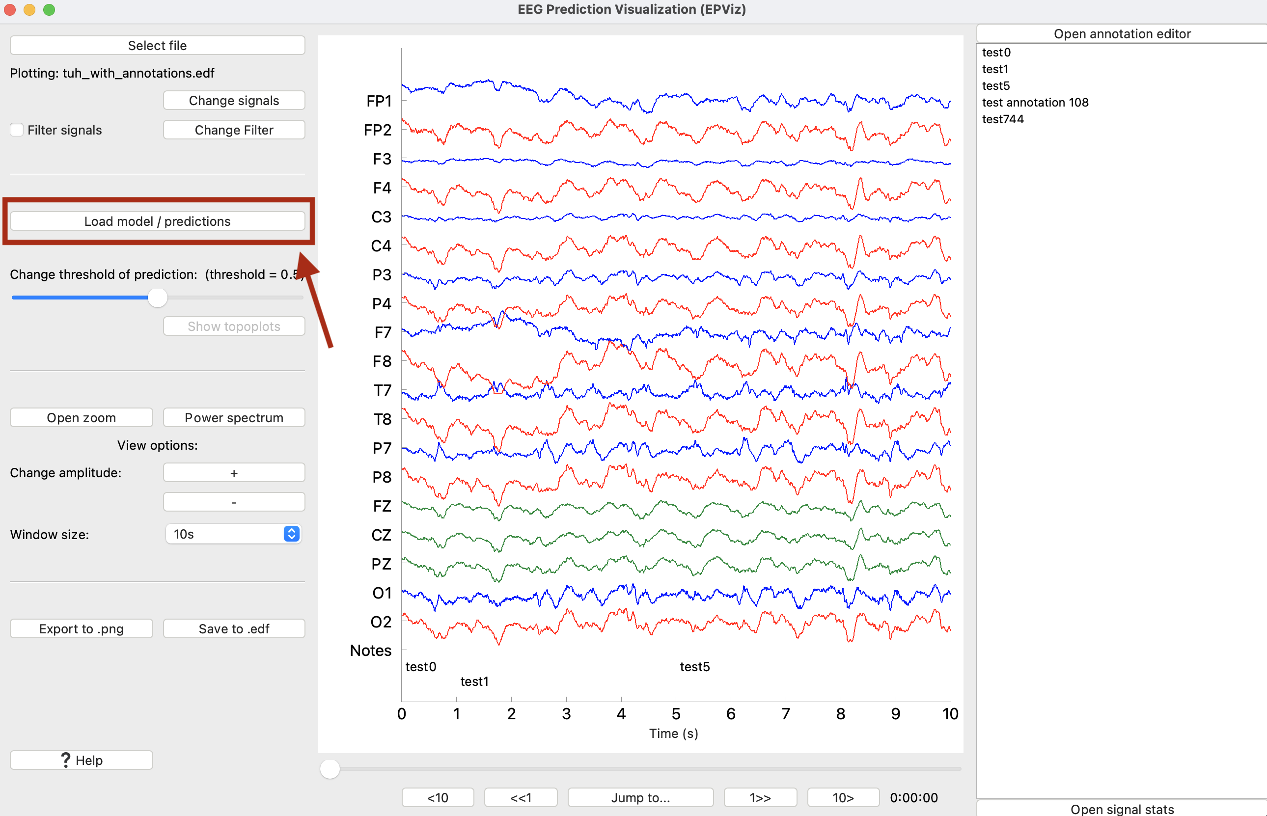

Predictions can be loaded as either a separate model and features file or as a standalone predictions file generated by an auxiliary model. In this demo, we will load a predictions file. Click “Load predictions” and then “Ok” to show the predictions.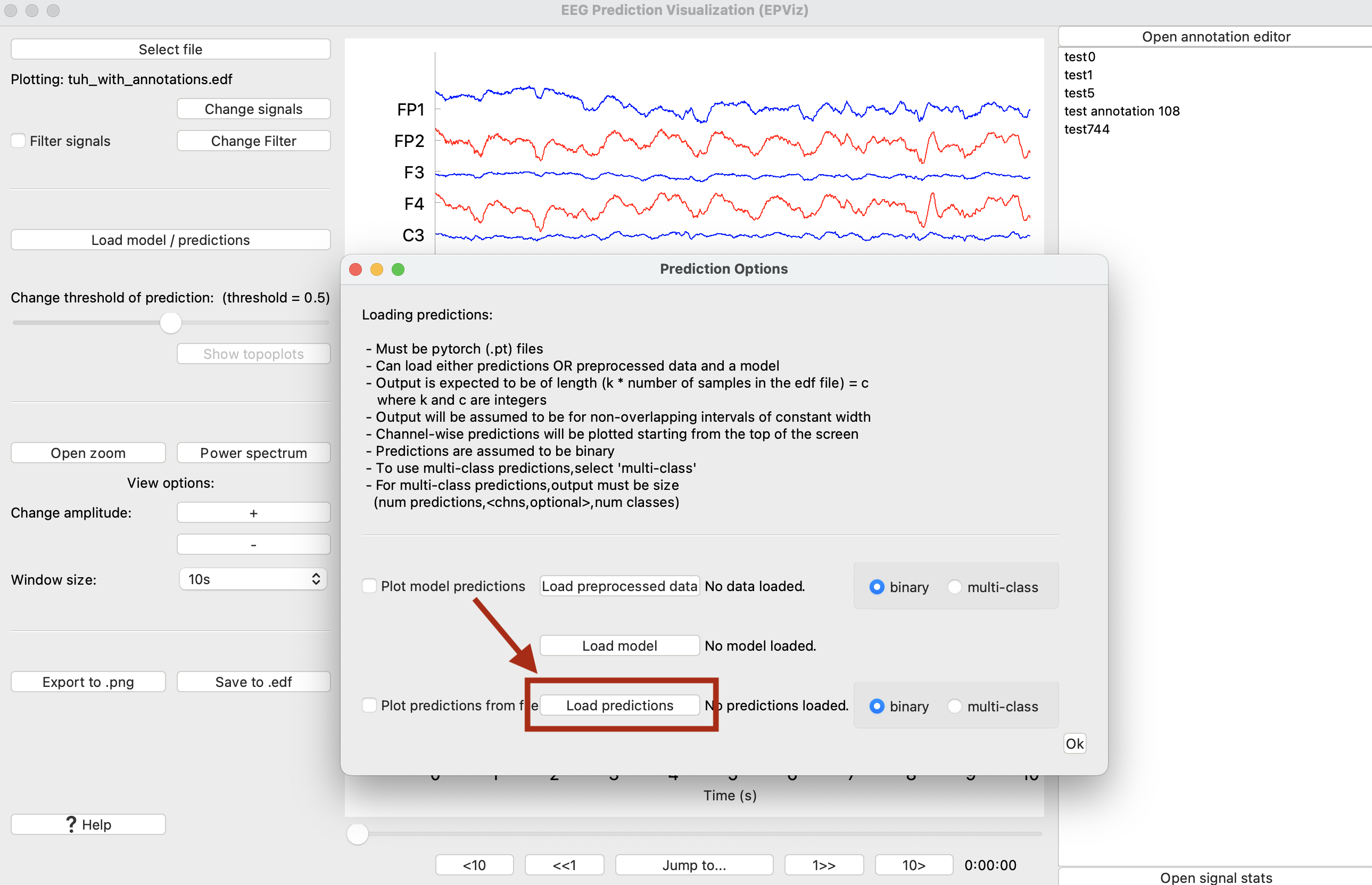

Since we have loaded multi-channel predictions, the topoplot window has been opened. Let’s scroll through the plot to see where the model has predicted a seizure. Scroll to 108 seconds in the plot. There are four different ways to accomplish this, numbered on the the plot below. You can (1) Use the “Jump to” button and type 108 to go to 108s, (2) Click the “10>” and “1>>” buttons to move in 10s and 1s increments respectively to reach 108s, (3) drag the slider to get to 108s, or (4) click on the “test annotation 108”.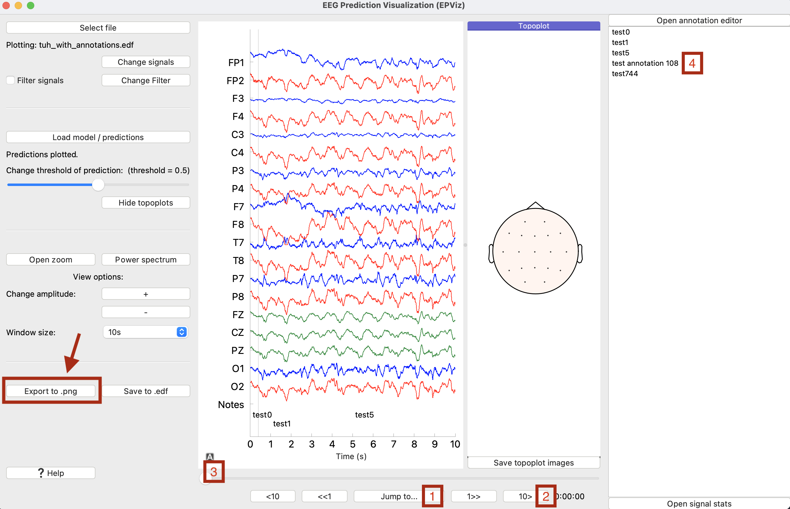

At 108s, we can see the model predictions highlighted in blue on the main window. Let’s save this image to a file by clicking “Export to .png”. This will open the figure editor. Customize the figure and click “Ok” to save to a PNG file.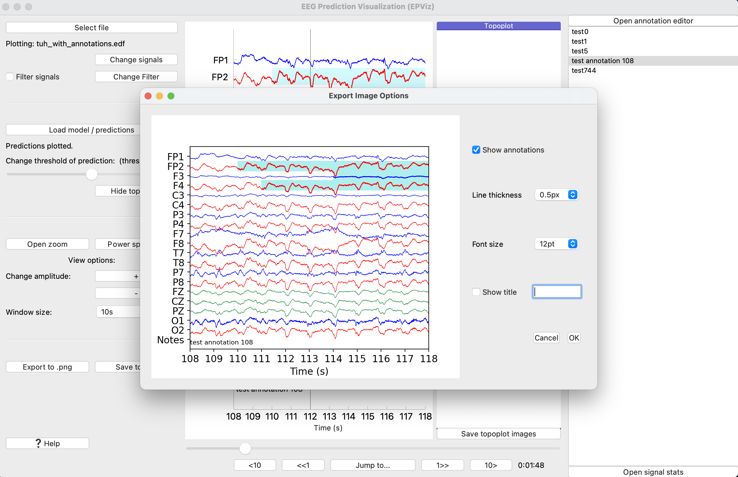

Finally, let’s save the signals and predictions to a new EDF file. Click “Save to .edf.” From here we can opt to keep the header the same or anonymize all fields. Suppose that we wanted to edit a couple of the fields. To do so, click “Edit header fields…”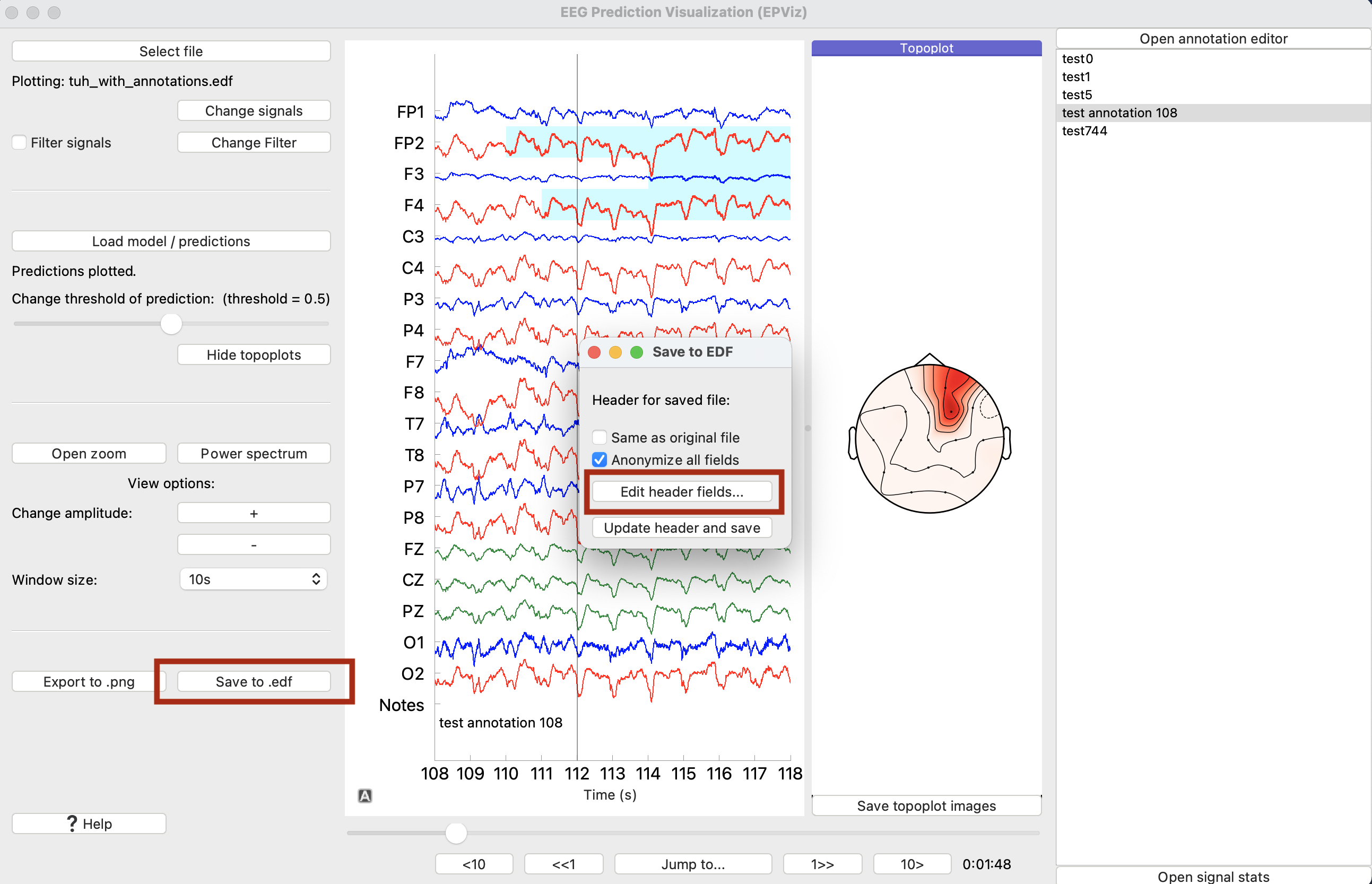

This opens the anonymization window. Here we can see the original fields and edit each field individually. Click “Anonymize and save file” to save your changes to a file.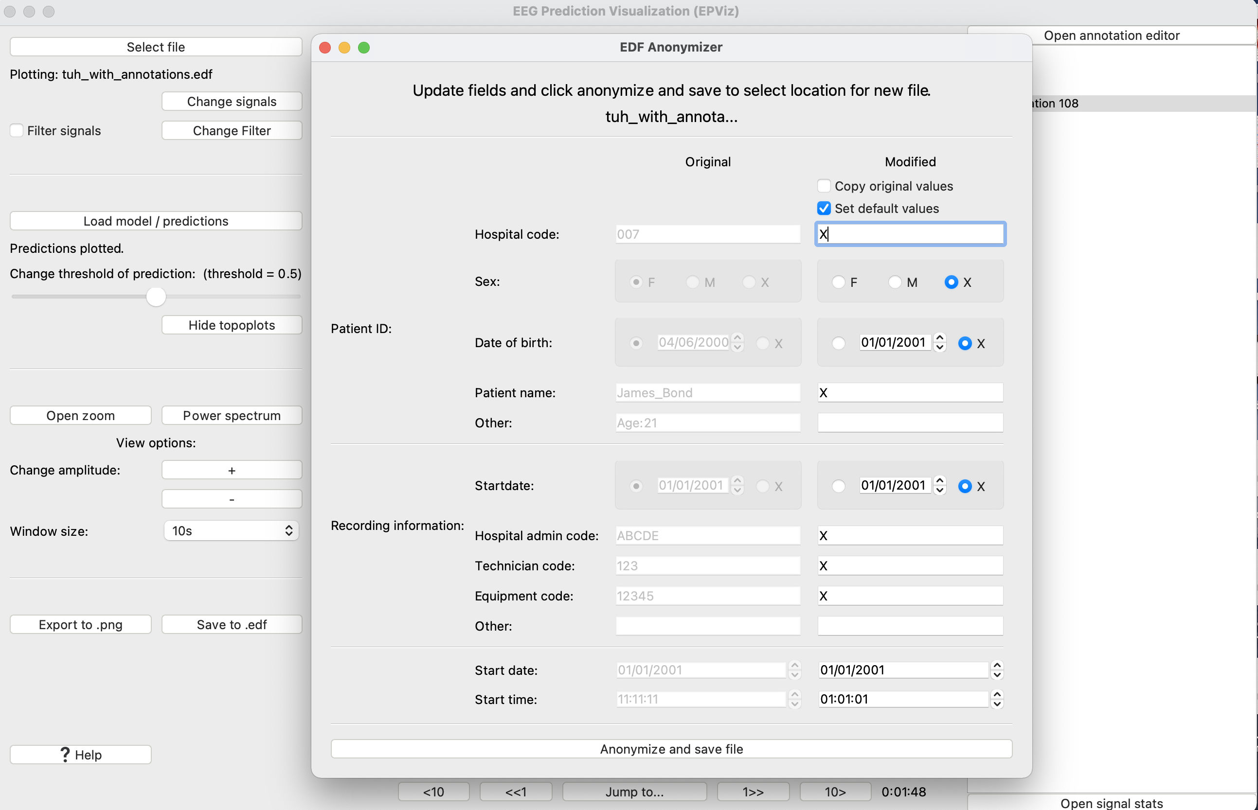

The new file will contain both the signals and the predictions that we plotted so they can be easily loaded for viewing in the future.

To report a bug, please create an issue here.

Neural Systems Analysis Laboratory

Decoding the Brain, One Snapshot at a Time

EPViz